October 1, 2025
E11 Bio Releases PRISM Technology for Self-Correcting Neuron Tracing
By Andrew C. Payne, Arlo Sheridan, Kathleen G.C. Leeper, Johan Winnubst
We share the PRISM platform for self-correcting neuron tracing using simple light microscopes. We describe a pilot study in mouse hippocampus and demonstrate how PRISM improves genetically labelled neuron tracing accuracy while adding molecular detail. We release a toolbox of constructs, methods, and data for research use.
Mapping the brain’s wiring with today’s tools is like navigating a black-and-white subway map with millions of tracks – the ultimate tracing problem. Yet finding a solution will transform neuroscience, and is critical for curing brain disorders, building safer and human-like AI, and even simulating brain function.
Today we are excited to release the full details of our PRISM neuron tracing platform – a major step towards solving this problem. The heart of PRISM is cell-filling tags (barcodes) that give each neuron a machine-readable identity, which is like adding 100,000 colors to the subway map. By combining barcodes with expansion microscopy and machine learning, PRISM boosts neuron tracing accuracy, bridges spatial gaps, and adds synapse-level molecular detail using accessible lab methods.
The work was conducted in partnership with the laboratories of Sam Rodriques (Francis Crick Institute, now Future House), Ed Boyden (MIT and HHMI), and Joergen Kornfeld (MPI).
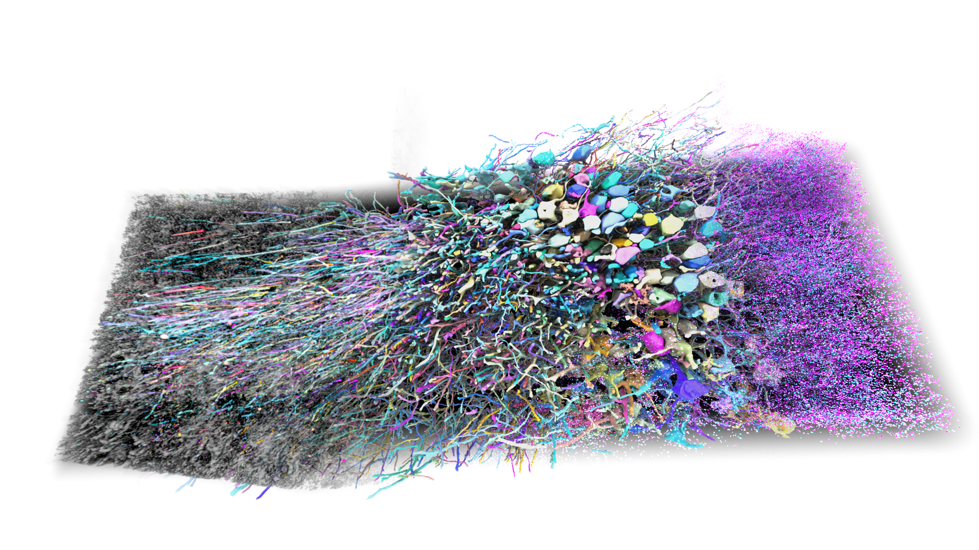
Video 1: Pilot study in mouse CA2/3 hippocampus denoting barcoded image volume and 3D reconstruction of traced neurons.
Problem: Neuron tracing is the key bottleneck for brain mapping
To transform neuroscience and cure brain disorders, build safe, brain-inspired AI, and simulate brains, we need detailed maps of brain wiring in mammals. The effort to study these neuronal connections - a field known as connectomics - is developing the technology needed to map all these physical connections at scale, with the ultimate goal of mapping the ~100 billion neurons in a human brain.
The effort to study neuronal connections and wiring is a field known as connectomics. It has the ultimate goal of mapping the ~100 billion neurons of human brains. On a practical level, the state of the art is slicing brain tissue into ultra-thin sections, imaging them sequentially at high resolution, stitching and aligning the many images back into 3D volumes, and then using AI to accurately trace each individual neuron through these large image volumes. The field is moving fast: we now have a full fruit-fly connectome (Dorkenwald, 2024) and millimeter-scale maps in mouse and human (Bae, 2025, and Shapson-Coe, 2024).
These triumphs, however, also revealed two key bottlenecks that currently prevent scaling up to a full mouse brain or beyond – and both center on tracing neurons.
Bottleneck 1: tracing accuracy. AI routinely gets confused when tracing neurons through large 3D volumes, either splitting single neurons into multiple pieces or incorrectly merging multiple neurons into one. A recent landmark study that comprehensively traced just ~1,500 mouse neurons required years of human revision and over a million manual fixes to the AI-generated map (Bae, 2025). While a monumental achievement, this implies a cost of tens of billions of dollars to trace a whole mouse brain (Scaling up Connectomics, 2023).
Bottleneck 2: robust sample processing. Tracing neurons over long distances is also exceptionally difficult because if ultra-thin brain sections are lost or damaged, the dataset gets split into discontinuous chunks (Bae, 2025). No one has successfully traced neurons through even 1 mm of sliced tissue in all three dimensions, and you’d need to do this ~500 times to complete a mouse brain connectome.
Opportunity: Light microscopy and cell barcodes offer a solution
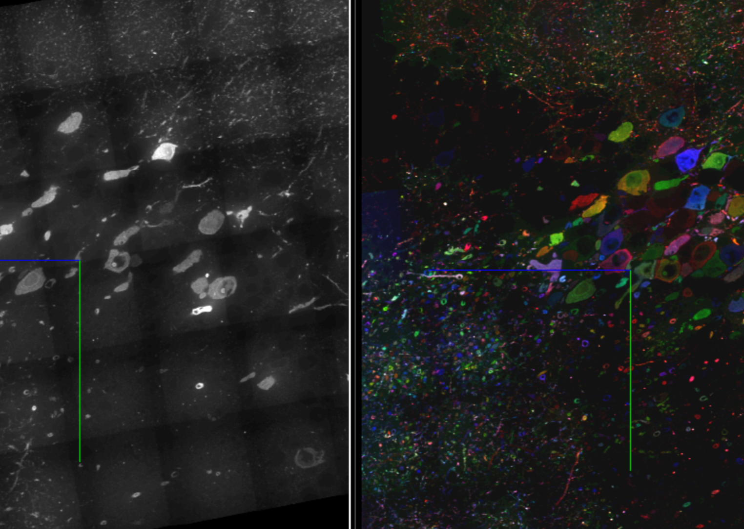
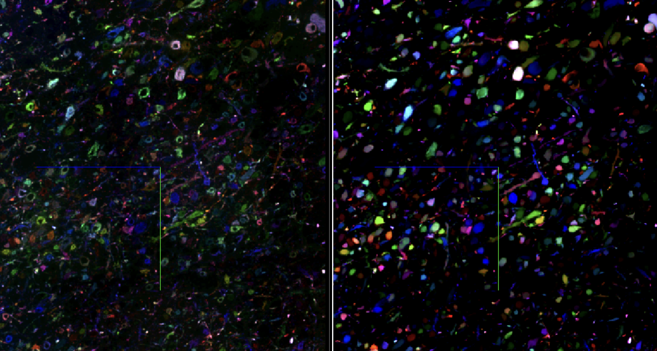
Why is tracing neurons so hard for AI or expensive for human proofreaders? Imagine planning a trip across an unfamiliar city with a subway map printed only in black-and-white. Where lines cross, it can be tough to tell which track belongs to which route. Transit planners found a solution to this by making each line a different color so you can easily follow the visually distinct path through crossings (Figure 1).
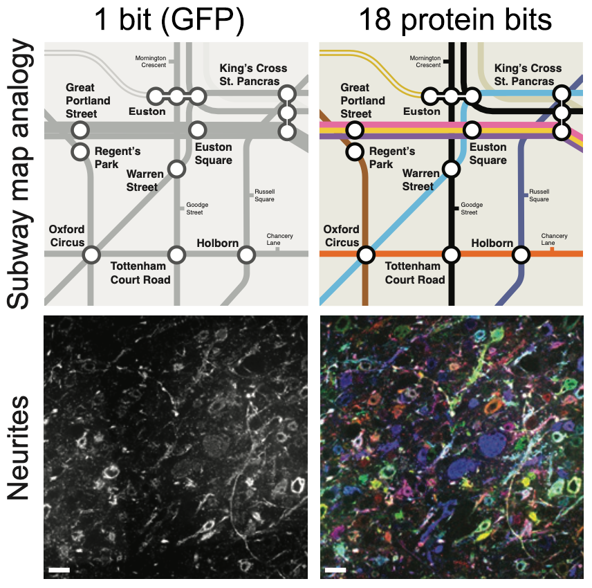
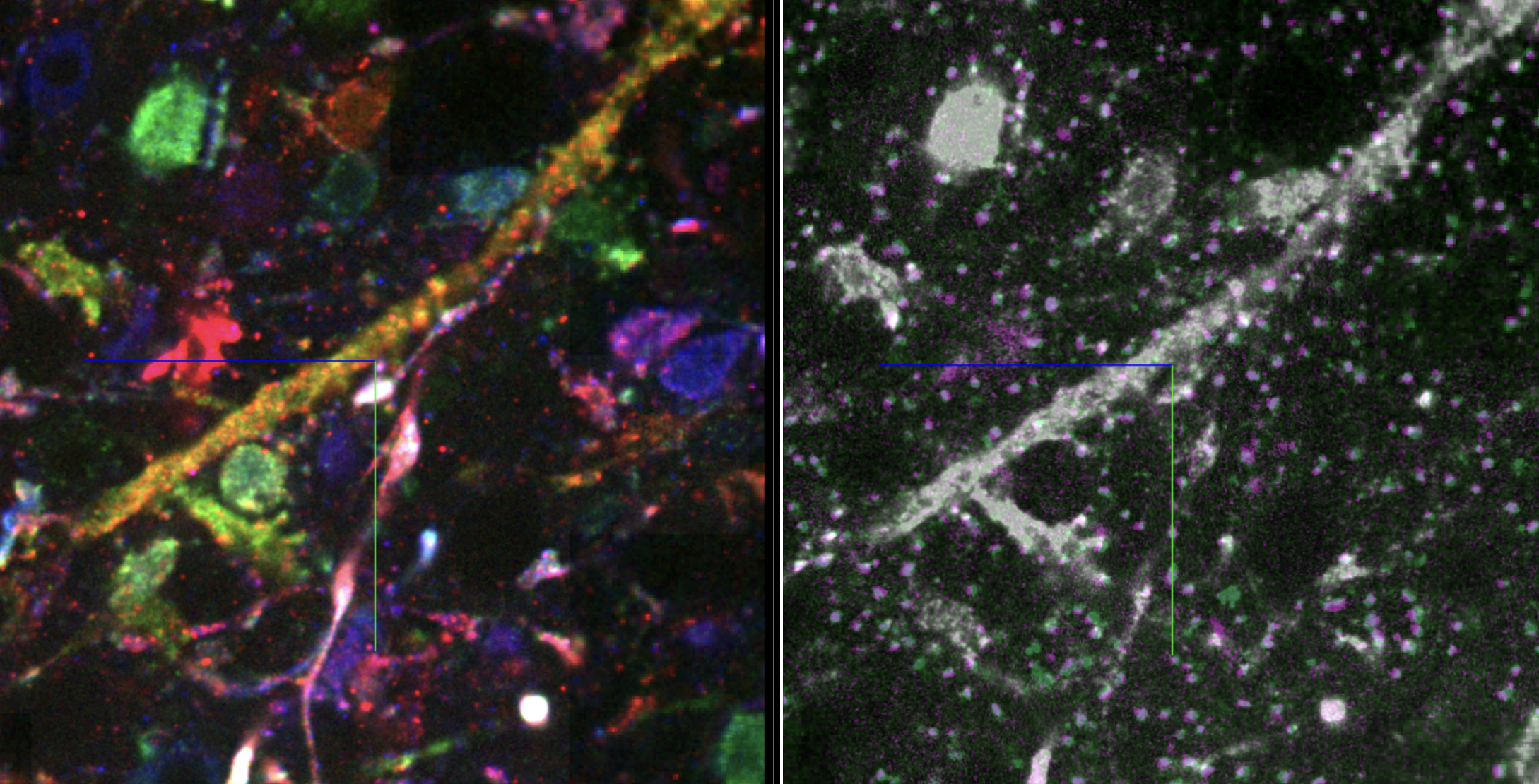
Figure 1: Subway map analogy illustrating the use of protein barcodes for automated segmentation. Top panels: Map from the London Underground. Bottom panels: Image of tissue from the hippocampal CA3 region. The left panels show single-color representations while the right panels display multiple channels or barcodes. Scale bar: 20 μm (pre-expansion).
Neuroscience has a version of this idea: make every cell a different color with fluorescent proteins (Livet, 2007; Sakaguchi, 2018). But this approach is limited to just a few hundred hues — nowhere near enough to label the millions or billions of neurons in mammalian brains.
Instead of using color, it is possible to give each cell a unique molecular tag — a cell barcode. In principle, barcodes scale far beyond the palette of distinguishable colors, approaching one unique label per cell. The catch is that nucleic acid barcodes aren’t abundant enough throughout the cell to act as continuous “paint” for tracing.
E11 Bio’s approach bridges the gap with protein barcodes: abundant, cell-filling tags that permit transit-style neuron tracing at the scale of molecular barcodes. In our paper, we estimate that our PRISM technology creates barcode diversity >750-fold greater than previous multicolor approaches while retaining strong cell-filling labelling.
In our paper, we prove the concept that protein barcodes help with neuron tracing. We leverage barcodes to directly improve image segmentation accuracy, and to reconnect neurons across the gaps, which is essential for robustness to missing or damaged tissue sections. These two factors are multiplicative and, in this first pilot study, we achieved an 8x improvement in tracing accuracy for genetically labelled neurons at high resolution.
We also show how PRISM can go beyond neuron tracing by annotating neurons with direct molecular measurements such as synapse composition, which is not practical in greyscale imaging. Critically, PRISM is accessible with conventional lab techniques and equipment. In this blog post we’ll explain how it works, preview the kinds of data it produces, and share resources – plasmids, reagent lists, protocols, and code – so you can use PRISM in your own research.
PRISM at a glance
Video 2: PRISM overview.
PRISM integrates several cutting-edge advances:
- Protein barcoding: At the heart of PRISM is the concept of cellular barcodes. Neurons are engineered to express a random subset of antigenically-distinct, cell-filling proteins (‘protein bits’). Thanks to the power of combinatorics, the palette of potential unique barcodes rapidly expands as the number of available proteins increases. With fluorescent proteins, there are ~27 = 128 possible binary combinations. In our paper, we demonstrate 18 bits (218 − 1 = 262,143 possible binary combinations).
- Expansion microscopy & iterative immunostaining: Expansion microscopy is a process where biological samples are embedded in a swellable gel matrix and then physically expanded to increase the effective imaging resolution. The sample is analyzed using round after round of antibody binding, imaging by light microscopy, and washing to remove the antibodies. The tissue expansion allows light microscopes to resolve nanometer-scale biological details that are usually only seen with electron microscopy. The repeated rounds of staining allow many different targets to be visualized in each cell. In our paper we image 23 targets: 18 protein bits and 5 molecular markers.
- Automatic neuron segmentation and proofreading: PRISM leverages our barcodes to improve neuron-tracing algorithms in three ways. First, the barcodes are used to sharpen the algorithm’s determination of boundaries of each neuron. Second, the barcodes are used in an automatic proofreading step, where the distinct barcodes help incorrectly-split neuron segments to be connected across gaps. By combining these factors, we show an 8x improvement in the error-free distance we can trace genetically labelled neurons.

Figure 2: Overview of PRISM technology. Protein Barcoding: Cells in brain tissue are barcoded as they receive random combinations of antigenically distinct proteins. Expansion Microscopy (and iterative staining): Tissue is expanded to improve imaging resolution resolution, and multiplexed through multiple rounds of antibody staining and imaging. AI reconstruction: The 3D structure of neurons is reconstructed by AI tools.
Key findings from our research
We acquired a unique dataset with PRISM in mouse CA2/3 hippocampus
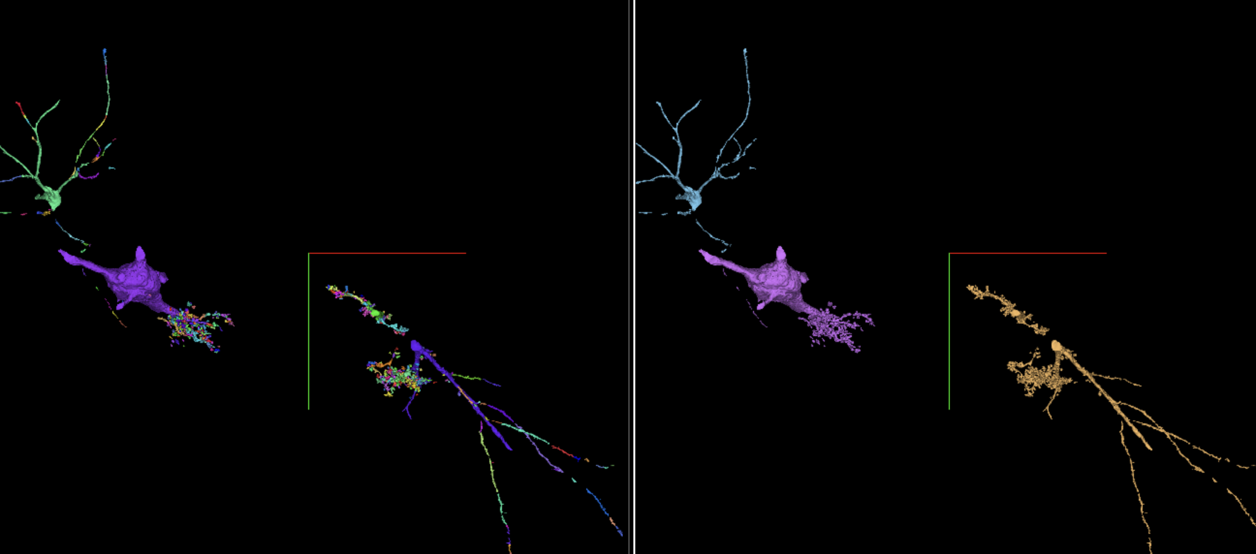
We demonstrated PRISM in a 10 million μm3 volume of hippocampus and showed that our iterative staining can detect 18 protein bits and 5 synaptic markers. The protein bits enabled automatic neuron segmentation and proofreading while the synaptic markers identified excitatory and inhibitory synapses (Figure 3).
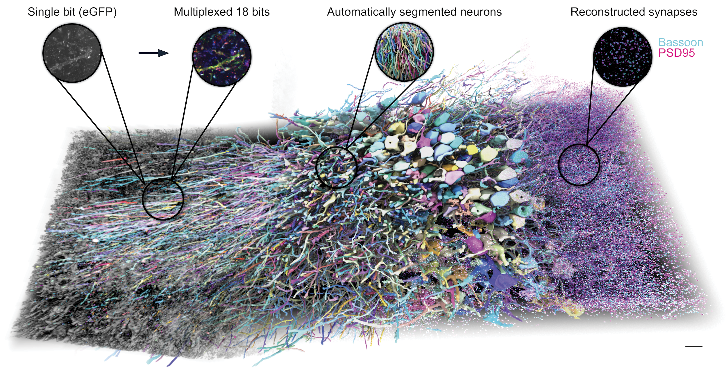
Figure 3: 3D rendering of a 10 million cubic micron volume of mouse hippocampal CA2/CA3 at a 35 x 35 x 80 nm voxel size. Colors from left to center demonstrate labeling of neurons with unique combinations of the 18 protein bits. Pink and cyan points at the right edge show synapses identified via stained synaptic markers. Enlarged circles at top (left to right) highlight four different aspects of the dataset: the first and second compare a grayscale (eGFP) single-plane image to the same multi-colored image labeled with 18 protein bits. The third demonstrates 3D neuron tracing segments using 18-bit protein barcodes. The fourth shows synapse reconstructions using the presynaptic active zone marker Bassoon and the postsynaptic excitatory scaffold protein PSD95. Scale bar: 10 µm pre-expansion.
We designed proteins that form combinatorial barcodes
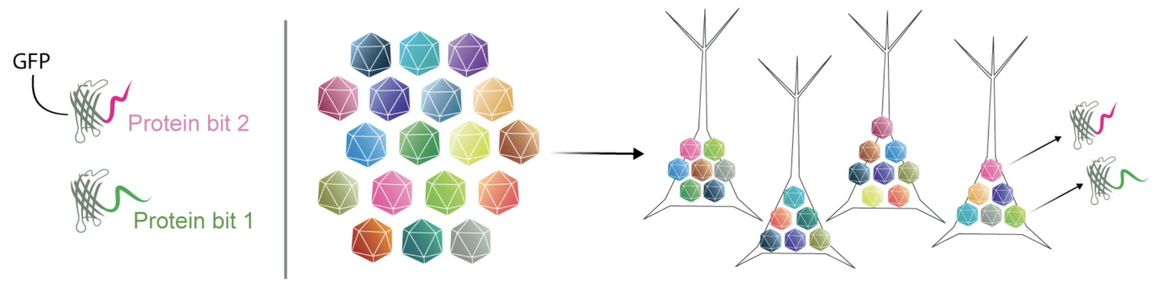
Figure 4: Structure of protein bits; combinatorial protein barcoding via stochastic AAV infection. Stochastic infection leads to the expression of random combinations of protein bits.
The key to our approach is a library of designed “protein bits”. Each protein variant represents a bit in a barcode, and are based on GFP proteins fused to short, antigenically distinct peptide tags. We designed 18 variants in total. We used a simple C-terminal fusion structure with minimal modification of the GFP, thus maintaining important characteristics of the base protein (i.e. cell-filling labelling). We created a pool of viruses (AAV), where each virus encodes one of these protein bits. When the pool is injected into the mouse brain, multiple viruses stochastically infect each neuron. Each cell thus expresses a subset of bits to create a protein barcode (Figure 4).
We developed iterative immunostaining methods for expanded tissue
After barcode injection, we expanded sliced tissue 5-fold, allowing an effective resolution of ~35 × 35 × 80 nm, fine enough to resolve dendritic spines, axons, and synapses. The expanded tissue was then put through seven rounds of staining, imaging, and stripping, with up to six targets in each round. One of the protein barcode channels was re-stained in each round so that the images could be aligned afterward to create the final image volume. PRISM implements a number of technical developments, including optimized gel chemistry and imaging parameters, for robust iterative staining and preservation of targets across rounds.
We generated diverse labels through successful stochastic barcoding
How well did the PRISM protein barcoding process perform in vivo? We quantified using the cell bodies in this dataset. Each of the 18 protein bits was present in ~20% of cells on average, and most neurons showed positive expression for 3-6 bits (Figure 5). This stochastic mixing yielded diverse barcodes: 80% of cells carried a unique barcode (different from all others by at least one bit). We estimated that we expressed 100,000 unique barcodes in this particular brain. This represents a ~750-fold improvement in diversity over previous multispectral labeling methods.
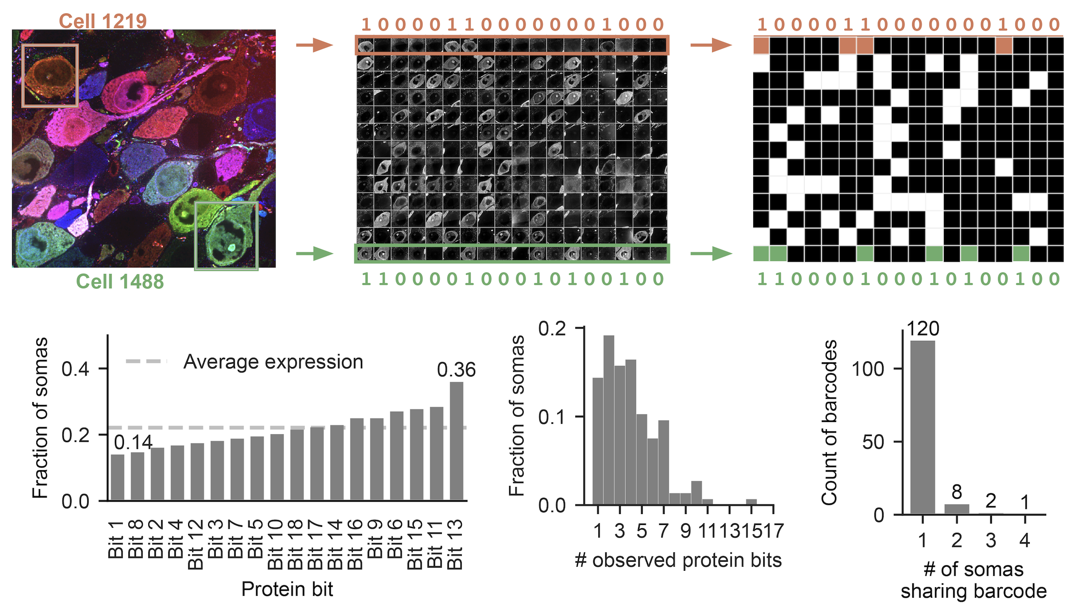
Figure 5: Barcode staining of cells. Top: Individual cells are classified into presence or absence for each protein bit to create a binary matrix. The image at left shows 13 cell bodies, the image at center shows the staining for the 13 cells (in rows) for the 18 protein bits (columns), the graph at right shows the binary result. Bottom: descriptive statistics across all somas in the dataset. The figure at left shows protein bit expression fractions. The center figure shows the distribution for the total number of expressed protein bits. The right figure quantifies the uniqueness of observed barcodes.
Interactive Figure 1: Interactive visualization of the 18 channel barcoded raw data. The left panel visualizes each channel individually (channels can be cycled through). The right panel shows all channels visualized with a multi-channel shader. Colors can be randomly cycled using seeds and the individual channel colors/intensities can be tuned. Tutorial. May load slowly.
We computationally improved the quality of barcode information
In order to capitalize on the benefits of diverse barcodes, we taught a network to diffuse the barcode signal throughout each cell, effectively teaching it to ‘paint-in’ an averaged barcode signal, thereby improving the signal quality and removing unwanted noise. To further improve barcode separability, we projected the enhanced barcodes into a uniform embedding space (Wang, 2020, Lee, 2021), making the barcodes more distinguishable from cell to cell (Figure 6).

Figure 6: We first “enhance” the barcodes by learning to predict the average barcode per neuron. We then project the enhanced barcodes (18 channels, ranging from 0 to 1) into a more uniform space (24 channels, ranging from -1 to 1). Images are RGB-color encoded for visualization.
Interactive Figure 2: Interactive visualization of raw (left) vs enhanced (right) barcodes. Tutorial. May load slowly.
We improved neuron tracing and segmentation by including barcode information
In order to generate neuron segmentations, we decided to use a standard affinity graph (Turaga et al., 2010) pipeline in which a network learns to predict boundaries (affinities) between distinct neurons. These affinities can be represented in a graph structure that can then be efficiently clustered (for example with mutex watershed; Wolf et al., 2018) to form unique segments. Such pipelines have now been scaled to run on petabyte-sized datasets (Macrina, 2021, Dorkenwald, 2024, Bae, 2025). While there are many favorable properties of affinity graphs for neuron segmentation, they have so far primarily been designed for grayscale data (e.g EM volumes), and therefore networks need to learn to deduce boundaries from the complex image textures, intensities, and shapes (Lee, 2017, Funke, 2019, Sheridan, 2022). A good overview can be seen in this blog post. We therefore wanted to incorporate the implicit “color” information provided by the barcodes. We were able to directly compute “barcode affinities” such that neighboring pixels within an object would have a high affinity weight, and pixels across objects would have a low affinity weight. We were then able to simply combine these barcode affinities with the traditional “shape affinities”, effectively making use of both shape and color information (Figure 7).
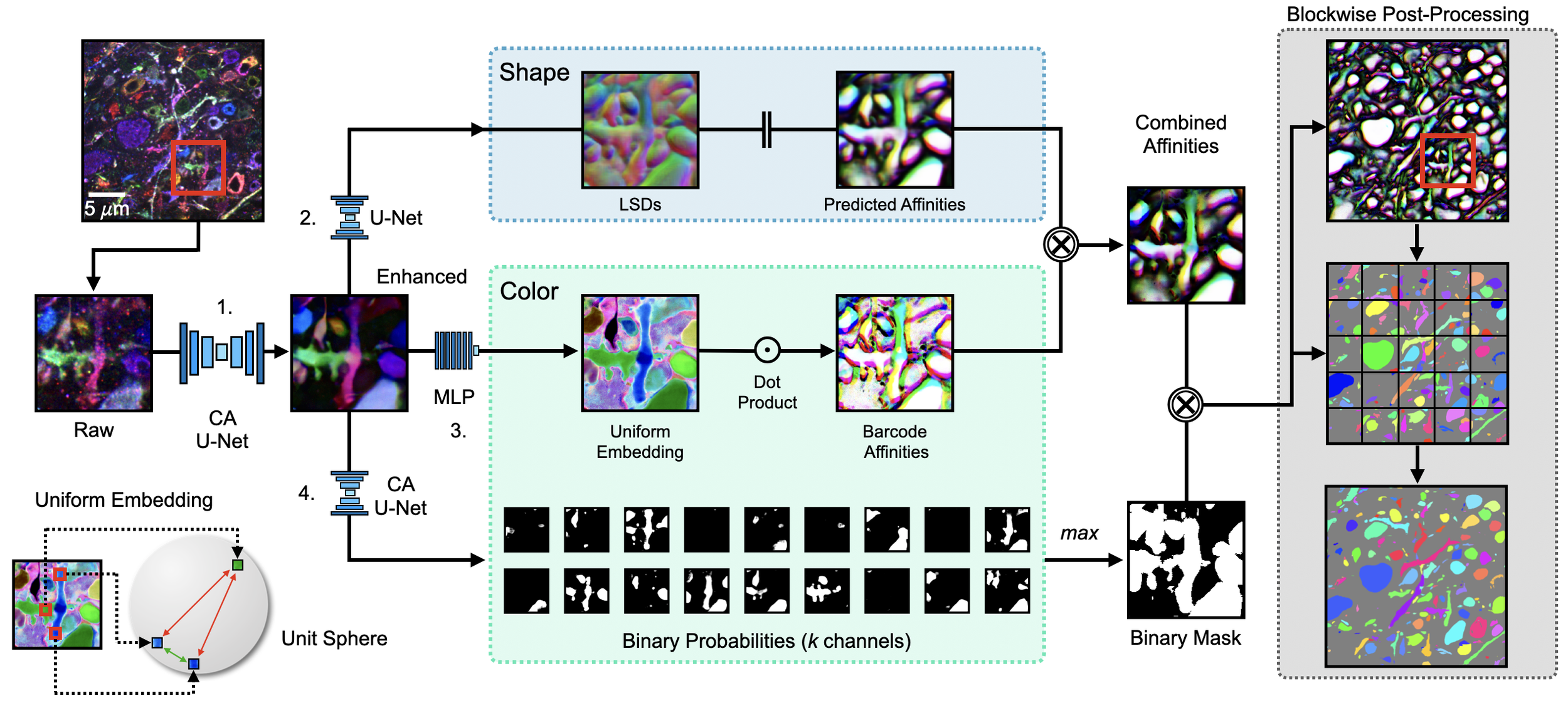
Figure 7: Overview of segmentation pipeline. Barcodes are enhanced and projected into a uniform space, and affinities are then computed from this embedding (via the dot product). Separately, we use the enhanced barcodes as input to a traditional shape-based affinity pipeline. We then combine these two affinities and use them as input to a blockwise segmentation pipeline. Additionally we use the barcodes to learn a binary mask of neurons in which barcodes are expressing, in order to prevent false merges against the background signal.
Importantly, this prevented false merges in segments between two neurons with distinct barcodes. To quantify accuracy improvements, we examined a number of metrics, including NERL (defined as the distance a neurite can be traced before making an error, normalized by the maximum possible run length), as well as NVOI (a commonly used metric to compare clusterings) and edits needed to correct the segmentation (described in more detail in the preprint, and in this paper). Incorporating barcodes into this process improved accuracy by 4x over the grayscale (GFP) baseline for NERL, and achieved 2-4x improvements across all metrics (Figure 8).
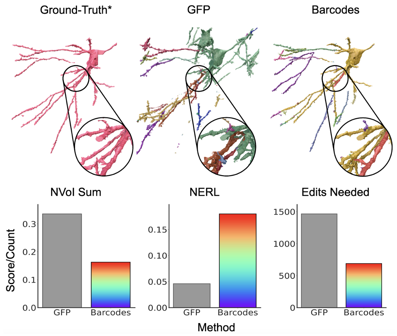
Figure 8: Barcodes help improve segmentation when used as input to affinity pipeline compared to grayscale (GFP) baseline. The top row shows an example ground truth neuron (a segment generated around a ground truth skeleton), and the corresponding segments from GFP and barcode affinity segmentations (>= 50% overlap with ground truth segment). The bottom row shows segmentation accuracy using common evaluation metrics.
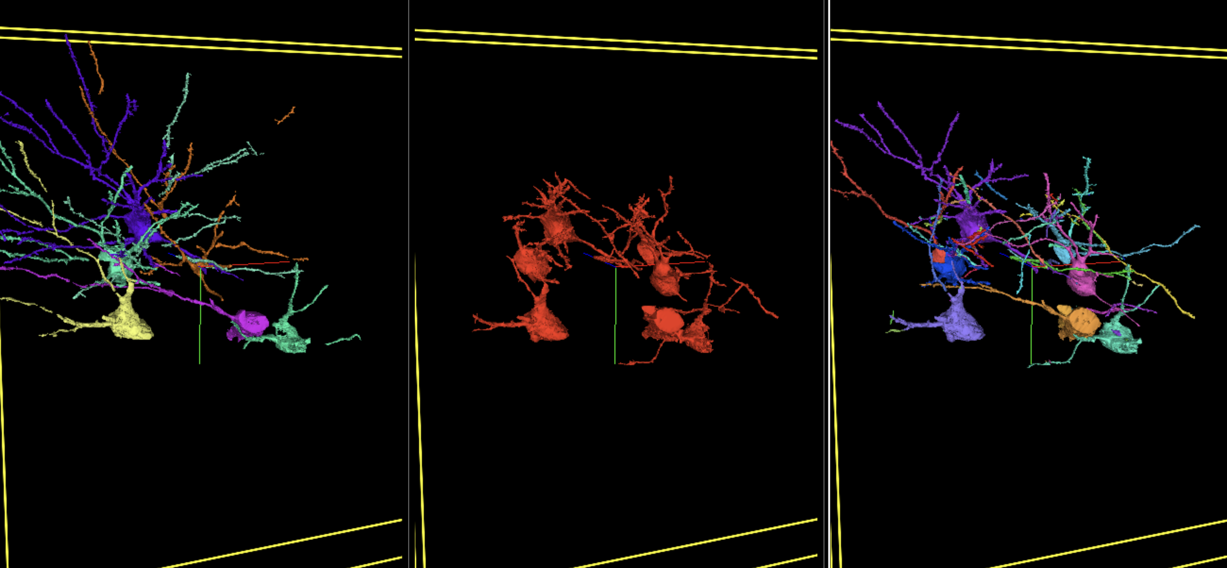
Interactive Figure 3: Interactive visualization of a subset of selected segments demonstrating how barcodes help to decrease false merges in initial affinity segmentation. Middle panel shows several falsely merged segments. Left panel shows overlapping (>=50%) “ground truth” segments. Right panel shows overlapping barcode affinity segments. Tutorial. May load slowly.
We leveraged barcodes for automatic proofreading
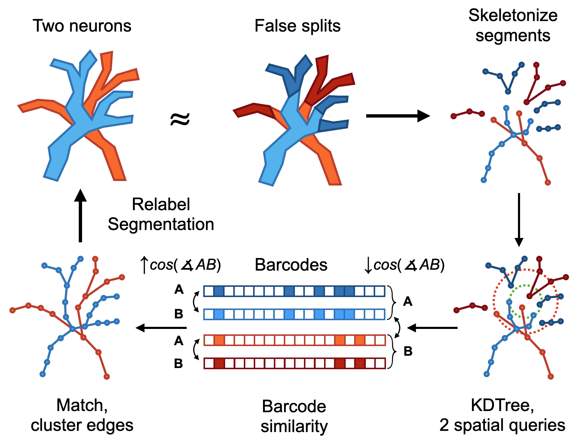
Figure 9: Overview of barcode relabeling strategy. Example shows two neurons in which the segmentation produced falsely split segments. We skeletonize these segments and assign the per-segment average barcode to the graph nodes. Then, in a spatial window, we compute edge weights based on the distance between barcodes. We then cluster these edges, and use the resulting lookup table to relabel the split segments. A nice feature about this approach is that the clustering and relabeling can be done in the same way as the affinity pipeline.
We hypothesized that barcode information could additionally be used in an “automatic proofreading” step following image segmentation to further improve accuracy. We computed each segment's average barcode to use as nodes in a graph where edge weights were assigned based on barcode similarity. Additionally, we constrained this spatially for efficiency and to prevent cascading merges which become more likely across larger distances. We were then able to cluster these edges (similar to what we did for the affinities), and relabel the segments from the affinity segmentation (Figure 9). This relabeling provided an additional ~2-4x increase across all accuracy metrics. Importantly, automatic proofreading allowed us to re-merge split segments across spatial gaps, and was multiplicative with segmentation improvements, achieving an 8x total improvement in run length accuracy (Figure 10). This is a promising approach for automatic proofreading, which could potentially be combined with global shape methods (Januszewski, 2025, Troidl, 2025) in the future. Critically, we observed that we could cross spatial gaps using barcodes, which is essential for overcoming sample robustness challenges such as lost or damaged tissue sections.
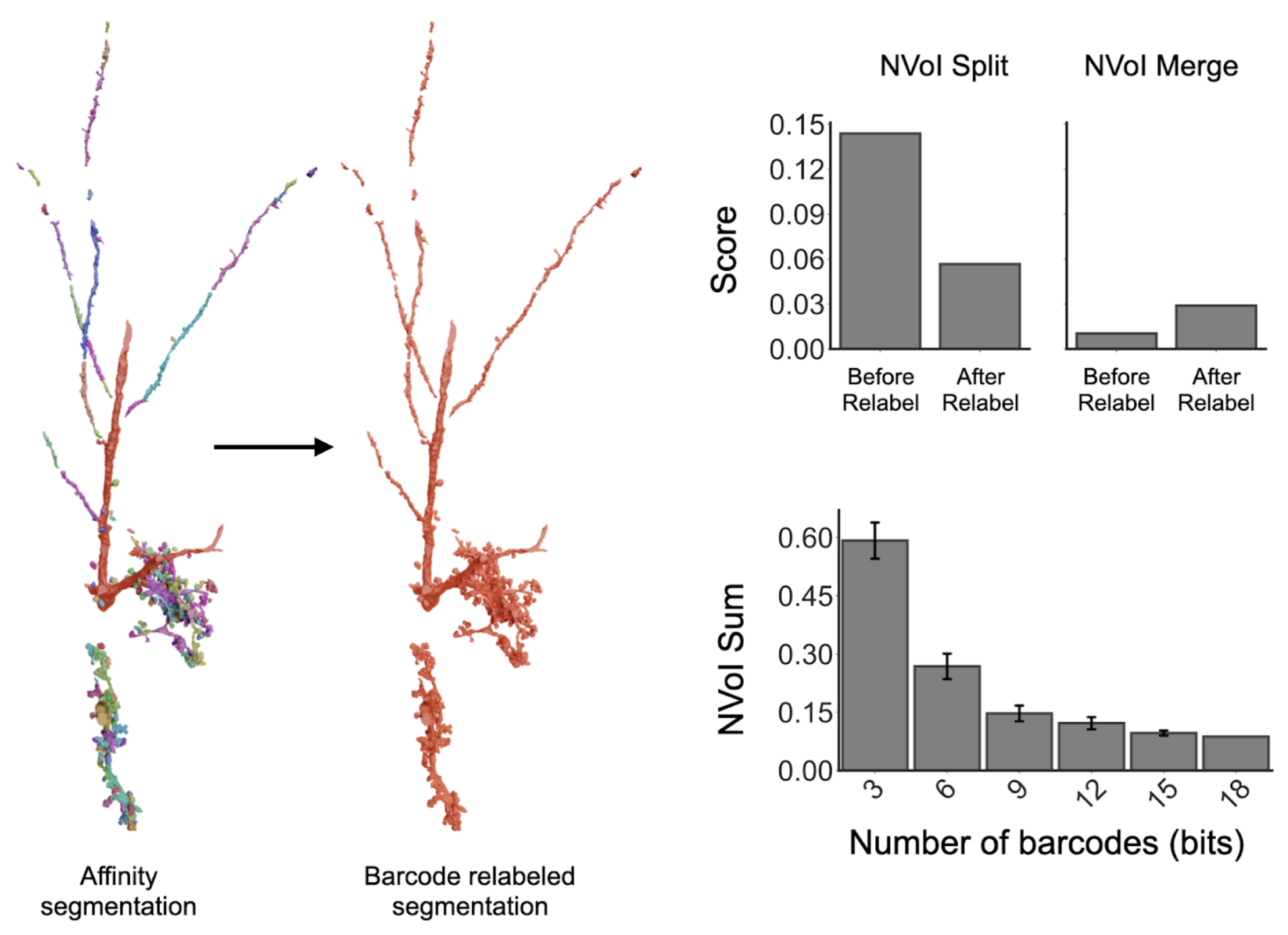
Figure 10: Example neuron with resulting mesh from the affinity segmentation and corresponding barcode-relabeled meshes. Barcodes allow for the main fiber to be reconnected alongside the complex dendritic bouton structures across spatial gaps. By relabeling the segments using barcodes, we were able to decrease the false split rate with minimal increases to the false merges (which are due to barcode collisions). Importantly, this accuracy increases with the number of barcodes used for matching.
Interactive Figure 4: Interactive visualization of a subset of barcode relabeled segments. Left panel shows barcode affinity segments (417) which belong to three neurons. While the barcodes help to decrease the false merges in the initial affinity segmentation, there are unavoidable false splits. Right panel shows resulting segments after relabeling these segments using the barcode information. Tutorial. May load slowly.
We annotated neurons with synaptic connections detected using molecular labels
Since PRISM relies on the detection of virally-introduced proteins to read out the barcode, it can readily be extended to detect endogenous proteins. In this dataset we labeled a set of 5 proteins that make up part of the synaptic machinery of both excitatory and inhibitory synapses. To showcase this capability we developed a ML segmentation pipeline that could, with high accuracy, detect putative excitatory synapses in our dataset by segmenting pairs of proteins present on each side of an excitatory synaptic connection: Bassoon (presynaptic) and PSD95 (postsynaptic). We detected a total of ~9 million synapses in our dataset, and could accurately assign the synapses to their respective neurons (Figure 11). By applying this approach to a set of proofread neurons we identified an increase in synaptic density as a function of distance from the soma which matches the known layered architecture of the hippocampal circuit. These findings show that PRISM can be used to investigate synaptic innervation patterns on the dendrite.
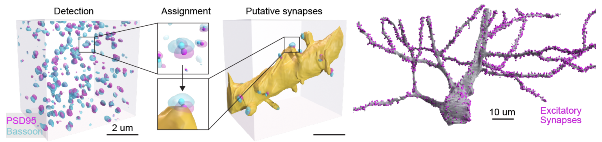
Figure 11: Schematic of ML synapse detection and assignment. Left: 3D volume of detected overlapping PSD95 (magenta) and Bassoon (cyan) labels. The center of each detected label is shown as a solid sphere. Center: a blown-up example pair of PSD95 and Bassoon labels alone, top, or assigned to a segmented neuronal morphology, bottom. Right: same 3D volume shown on the left but only showing label markers that could be assigned to the dendrite rendered in yellow. Right: Example of a proofread pyramidal neuron with assigned excitatory synapses (magenta).
We uncovered new properties of the nanostructural organization of synaptic connections
The expansion microscopy approach used by PRISM allows us to resolve small morphological details that are normally obscured in conventional light microscopy. This was evident in the fact that we observed elaborate synaptic complexes known as ‘thorny excrescences’ that are formed on the dendrites of pyramidal neurons where they contact mossy fiber axons. Importantly, due to the previously mentioned molecular labeling we were able to identify the functional postsynaptic densities on these structures. Since these synapses have mostly been studied using limited EM data we decided to study them in more detail. We found that they were highly diverse in both volume and in the number of postsynaptic densities that they contained but that both properties were highly correlated (R2=0.90). We also observed an intriguing relationship where the volumes of nearby thorny excrescences on the same dendrite were significantly correlated (R2=0.37) suggesting a potential spatially-clustered organization (Figure 12). Together, these results show how PRISM can be used to drive systematic discovery.

Figure 12: Example of a thorny excrescence on a CA3 dendrite. Top left: Composite image showing a single protein-bit channel (gray), PSD95 (magenta), and Bassoon (cyan) antibody labeling. Top right: 3D reconstruction of the same stretch of dendrite. The arrow highlights the location of the thorny excrescence (TE) shown on the left. Bottom center: The volume of the TEs mapped on a single dendrite encoded by color. Bottom left: Observed correlation between TE volume and the number of detected postsynaptic densities. Bottom right: Observed correlation between each TE’s volume and the volume of TEs on the same dendrite within 5 μm. Gray dashed lines indicate the best-fit linear regression. Statistical significance is given as r=Pearson correlation coefficient, ***: p<0.001.
Interactive Figure 5: Interactive visualization of raw barcodes using multichannel shader (left), and channel-wise (right). Right panel also shows bassoon and PSD95 markers. Tutorial. May load slowly.
Next Steps
E11 Bio’s mission is to transform neuroscience through mammalian connectomics, which means overcoming key bottlenecks holding back the field. Two issues dominate: automated AI tracing still makes too many mistakes, and sample defects can prevent tracing altogether. PRISM tackles both while adding molecular annotation to neuron reconstructions.
We’re excited about what comes next. Because PRISM is an open toolbox, individual labs can use it to incorporate barcoding, accessible neuron tracing analysis, and molecular annotation into everyday neuroscience without specialized equipment or compute resources. All neuron tracers stand to immediately benefit, as well as diverse applications spanning barcoded viral gene delivery, lineage tracing, and cell therapies.
There are exciting near-term opportunities to build on this foundation, expand the capabilities of PRISM, and leverage self-correcting neuron tracing. Integrating PRISM with ultrastructure labeling (Damstra, 2023, M’Saad 2022, Tavakoli, 2025) would permit self-correcting neuron tracing to be extended to the field of connectomics, where limitations of tracing accuracy and sample defects are felt most acutely. Next steps could also include incorporating PRISM with other mutually supportive advances in AI tracing (Troidl, 2025, Januszewski, 2025). And we have just scratched the surface of what is possible with protein barcodes. Due to exponential scaling, doubling the number of protein bits using new generative AI protein design methods (Cao, 2022) would unlock billions of combinations for whole-brain barcoding. Through a combination of these factors, we see a clear path to connectomics at 100x lower cost – with transformative implications for neuroscience.
If you’re as excited about PRISM as we are, here are a few ways you might get involved:
Join us – we are hiring at multiple levels!
Try PRISM – we are interested in working closely with early adopters of PRISM as co-development partners.
Therapeutics and AI applications – we are particularly interested in exploring opportunities for self-correcting neuron tracing to help advance these areas. Ask us for a seminar or a conversation.
Follow our progress – sign up for our mailing list here.
How Can I Use PRISM?
We designed PRISM to be a toolbox accessible to any laboratory without the need for specialized equipment beyond a fluorescence microscope. In addition, we anticipate that the individual components of PRISM may be unbundled for diverse applications. Here’s are ways to access elements of the PRISM toolbox:
Protocols Our preprint includes detailed descriptions of methods and protocols, including expansion microscopy with iterative immunostaining. Access Preprint |
DNAOur PRISM collection of barcoding plasmids is available on Addgene, including an additional collection of Cre-dependent, neuron-specific plasmids useful for mapping specific circuits. Access Addgene |
Code Volara is an open-source Python library that facilitates the application of common block-wise operations for image processing of large volumetric microscopy datasets. Example network training code is available in this Github repo. |
Data A collection of data resources are available through the AWS Open Data program, including raw light microscopy images, segmentations, precomputed, & training data. This repo explains the data and has a couple download tutorials. Have a look at the available data by browsing our interactive Neuroglancer gallery! Access on AWS |
Acknowledgements
We partnered with the laboratories of Sam Rodriques (Francis Crick Institute, now Future House), Ed Boyden (MIT and HHMI), and Joergen Kornfeld (MPI) for this study. E11 Bio led experimental and computational development of methods, and processed and analyzed the hippocampal image dataset. Sam Rodriques and Sung Yun Park led acquisition of the image dataset and collaborated on methods. All partners contributed to conceptualization and early methods development.
For the preprint, Sung Yun Park led data acquisition, and Arlo Sheridan led development of barcode-augmented segmentation and automatic proofreading with support from William Patton. Kathleen Leeper led development of the protein barcodes, Sven Truckenbrodt led expansion microscopy development with support from Erin Jarvis, and Johan Winnubst led image registration and synapse analysis with support from Julia Lyudchik.
A full list of all author contributions can be found in the preprint, and we gratefully acknowledge all preprint co-authors: Sung Yun Park, Arlo Sheridan, Bobae An, Erin Jarvis, Julia Lyudchik, William Patton, Jun Y. Axup, Stephanie W. Chan, Hugo G.J. Damstra, Daniel Leible, Kylie S. Leung, Clarence A. Magno, Aashir Meeran, Julia M. Michalska, Franz Rieger, Claire Wang, Michelle Wu, George M. Church, Jan Funke, Todd Huffman, Kathleen G.C. Leeper, Sven Truckenbrodt, Johan Winnubst, Joergen M.R. Kornfeld, Edward S. Boyden, Samuel G. Rodriques, Andrew C. Payne. Full contributions detailed in preprint.
Figures by Julia Kuhl. Video by Jeroen Claus and Ethan MacKenzie, Phospho. Image rendering by Tyler Sloan, Quorumetrix Studio.
References
Bae, J. A., Baptiste, M., Baptiste, M. R., Bishop, C. A., Bodor, A. L., Brittain, D., Brooks, V., Buchanan, J., Bumbarger, D. J., Castro, M. A., Celii, B., Cobos, E., Collman, F., da Costa, N. M., Danskin, B., Dorkenwald, S., Elabbady, L., Fahey, P. G., Fliss, T.,... The MICrONS Consortium. (2025). Functional connectomics spanning multiple areas of mouse visual cortex. Nature, 640(8058), 435–447. https://doi.org/10.1038/s41586-025-08790-w
Cao, L., Coventry, B., Goreshnik, I., Huang, B., Sheffler, W., Park, J. S., Jude, K. M., Markovic, I., Kadam, ́R. U., Verschueren, K. H. G., Verstraete, K., Walsh, S. T. R., Bennett, N., Phal, A., Yang, A., Kozodoy, L., DeWitt, M., Picton, L., Miller, L., . . . Baker, D. (2022). Design of protein-binding proteins from the target structure alone. Nature, 605(7910), 551–560. https://doi.org/10.1038/s41586-022-04654-9
Damstra, H. G. J., Passmore, J. B., Serweta, A. K., Koutlas, I., Burute, M., Meye, F. J., Akhmanova, A., & Kapitein, L. C. (2023). GelMap: Intrinsic calibration and deformation mapping for expansion microscopy. Nature Methods, 20(10), 1573–1580. https://doi.org/10.1038/s41592-023-02001-y
Dorkenwald, S., Matsliah, A., Sterling, A. R., Schlegel, P., Yu, S.-c., McKellar, C. E., Lin, A., Costa, M., Eichler, K., Yin, Y., Silversmith, W., Schneider-Mizell, C., Jordan, C. S., Brittain, D., Halageri, A., Kuehner, K., Ogedengbe, O., Morey, R., Gager, J.,... Murthy, M. (2024). Neuronal wiring diagram of an adult brain. Nature, 634(8032), 124–138. https://doi.org/10.1038/s41586-024-07558-y
Funke, J., Tschopp, F., Grisaitis, W., Sheridan, A., Singh, C., Saalfeld, S., & Turaga, S. C. (2019). Large Scale Image Segmentation with Structured Loss Based Deep Learning for Connectome Reconstruction. IEEE Transactions on Pattern Analysis and Machine Intelligence, 41(7), 1669–1680. https://doi.org/10.1109/TPAMI.2018.2835450
Januszewski, M., Templier, T., Hayworth, K., Peale, D., & Hess, H. (2025, May). Accelerating Neuron Reconstruction with PATHFINDER [Pages: 2025.05.16.654254 Section: New Results]. https:// doi.org/10.1101/2025.05.16.654254
Lee, K., Zung, J., Li, P., Jain, V., & Seung, H. S. (2017, May). Superhuman Accuracy on the SNEMI3D Connectomics Challenge [arXiv:1706.00120 [cs]]. https://doi.org/10.48550/arXiv.1706.00120
Lee, K., Lu, R., Luther, K., & Seung, H. S. (2021). Learning and Segmenting Dense Voxel Embeddings for 3D Neuron Reconstruction. IEEE Transactions on Medical Imaging, 40(12), 3801–3811. https://doi.org/10.1109/TMI.2021.3097826
Livet, J., Weissman, T. A., Kang, H., Draft, R. W., Lu, J., Bennis, R. A., Sanes, J. R., & Lichtman, J. W. (2007). Transgenic strategies for combinatorial expression of fluorescent proteins in the nervous system. Nature, 450(7166), 56–62. https://doi.org/10.1038/nature06293
M’Saad, O., Kasula, R., Kondratiuk, I., Kidd, P., Falahati, H.,Gentile, J. E., Niescier, R. F., Watters, K., Sterner, R. C., Lee, S., Liu, X., Camilli, P. D., Rothman, J. E., Koleske, A. J., Biederer, T., & Bewersdorf, J. (2022, April). All-optical visualization of specific molecules in the ultrastructural context of brain tissue [Pages: 2022.04.04.486901 Section: New Results]. https://doi.org/10.1101/2022.04.04.486901
Macrina, T., Lee, K., Lu, R., Turner, N. L., Wu, J., Popovych, S., Silversmith, W., Kemnitz, N., Bae, J. A., Castro, M. A., Dorkenwald, S., Halageri, A., Jia, Z., Jordan, C., Li, K., Mitchell, E., Mondal, S. S., Mu, S., Neho- ran, B., . . . Seung, H. S. (2021, August). Petascale neural circuit reconstruction: Automated methods [Pages: 2021.08.04.455162 Section: New Results]. https://doi.org/10.1101/2021.08.04.455162
Sakaguchi, R., Leiwe, M. N., & Imai, T. (2018). Bright multi-color labeling of neuronal circuits with fluorescent proteins and chemical tags. Elife, 7. https://doi.org/10.7554/eLife.40350
Scaling up Connectomics - Reports. (2023, June). Retrieved August 5, 2025, from https://wellcome.org/reports/scaling-connectomics
Shapson-Coe, A., Januszewski, M., Berger, D. R., Pope, A., Wu, Y., Blakely, T., Schalek, R. L., Li, P. H., Wang, S., Maitin-Shepard, J., Karlupia, N., Dorkenwald, S., Sjostedt, E., Leavitt, L., Lee, D., Troidl, J., Collman, F., Bailey, L., Fitzmaurice, A., . . . Lichtman, J. W. (2024). A petavoxel fragment of human cerebral cortex reconstructed at nanoscale resolution. Science, 384(6696), eadk4858. https://doi.org/10.1126/science.adk4858
Sheridan, A., Nguyen, T. M., Deb, D., Lee, W.-C. A., Saalfeld, S., Turaga, S. C., Manor, U., & Funke, J. (2022). Local shape descriptors for neuron segmentation [Pub- lisher: Nature Publishing Group]. Nature Methods, 20(2), 295–303.https://doi.org/10.1038/s41592-022-01711-z
Tavakoli, M. R., Lyudchik, J., Januszewski, M., Vistunou, V., Agudelo Duenas, N., Vorlaufer, J., Sommer, C., Kreuzinger, C., Oliveira, B., Cenameri, A., Novarino, G., Jain, V., & Danzl, J. G. (2025). Light-microscopy-based connectomic reconstruction of mammalian brain tissue. Nature, 642(8067), 398–410. https://doi.org/10.1038/s41586-025-08985-1
Troidl, J., Knittel, J., Li, W., Zhan, F., Pfister, H., & Turaga, S. (2025, June). Global Neuron Shape Reasoning with Point Affinity Transformers [Pages: 2024.11.24.625067 Section: New Results]. https://doi.org/10.1101/2024.11.24.625067
Turaga, S. C., Murray, J. F., Jain, V., Roth, F., Helmstaedter, M., Briggman, K., Denk, W., & Seung, H. S. (2010). Convolutional Networks Can Learn to Generate Affinity Graphs for Image Segmentation. Neural Computation, 22(2), 511–538. https://doi.org/10.1162/neco.2009.10-08-881
Wang, T., & Isola, P. (2020). Understanding Contrastive Representation Learning through Alignment and Uniformity on the Hypersphere [ISSN: 2640-3498]. Proceedings of the 37th International Conference on Machine Learning, 9929–9939. Retrieved August 5, 2025, from https://proceedings.mlr.press/v119/wang20k.html
Wolf, S., Pape, C., Bailoni, A., Rahaman, N., Kreshuk, A., Kothe, U., & Hamprecht, F. (2018). The Mutex Watershed: Efficient, Parameter-Free Image Partitioning, 546–562. Retrieved August 5, 2025, from https://openaccess.thecvf.com/content_ECCV_2018/html/Steffen_Wolf_The_Mutex_Watershed_ECCV_2018_paper.html